Excel

Working with Data in Excel

Bookmark this page to return to it with ease.

Download Companion Excel Sheet

Position your windows so the spreadsheet takes up half your screen and this guide takes up the other half.

Table of Contents:

• Getting Started
• Functions
• Dropdown Menus
• Common Problems
  • Delimiters
  • Filling Blanks
• VLOOKUP
• PivotTables

Instructional videos are linked at the beginning of each of the five sections. Please list questions on this page for the discussion meeting.

Getting Started

Module 1 Video: Getting Started (16:19 minutes)

(View the first sheet of the Excel_Workshop spreadsheet.)

Shortcuts

To…	Windows	Mac
Find and replace	CTRL+F	⌘+F
Move to the edge of the data region	CTRL+Arrow key	⌘+Arrow key
Select to the edge of the data region	CTRL+SHIFT+Arrow key	⌘+SHIFT+Arrow key
Select entire column	CTRL+SPACEBAR	CTRL+SPACEBAR
Select entire row	SHIFT+SPACEBAR	SHIFT+SPACEBAR
Enter value into all selected cells*	CTRL+ENTER	⌘+RETURN

*Highlight empty cells; click into the formula bar above your data; type the value you want to enter in all of them; press the shortcut keys.

We’ll come back to this last shortcut—it’s useful and we’ll cover it in more detail, but it’ll make more sense when you see the example in the spreadsheet.

Best Practices and Tidy Data

• Each row is as an “observation” at a consistent level (e.g. no totals mixed in)
• Each column as a “variable” or “field”.
  • Don’t store more than one piece of information in a cell.
• Avoid color or other formatting alone to encode data.
• Only one table per sheet.
• Blank cells indicate missing values, zeroes indicate observed zeroes.
• Comments or notes should be integrated as a separate column or stored separately.

Consider this example of data collected about observed small mammals in desert research plots (from Data Carpentry’s Lesson for Ecologists, Formatting Data Tables in Spreadsheets section). How could things go wrong with the data presented this way? Try to think of at least two ways.

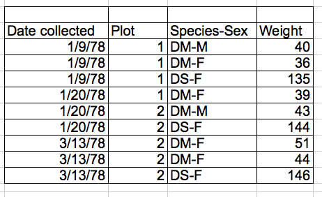
Try saving your data as a .csv (common separate values) file. This saves just the active sheet without formatting.

Functions

Module 2 Video: Functions (23:06 minutes)

Using Functions in Excel

(View the Functions sheet of the spreadsheet.)

• =SUM()
• =AVERAGE()
• =MEDIAN()
• Etc.

Working with Text

If you find you need to reformat observations, here are some functions that can help.

• =LEFT() Extracts a specified number of characters from a variable, counting from the left
  • =RIGHT() same as above, but counting from the right
• =TRIM() Removes all whitespace aside from single spaces between words
• =CONCATENATE() or =CONCAT() combines multiple cells of text into a single text cell
• Advanced exercise: logical function, IF
  If you’re used to logical functions, give this exercise a try. The solution is available in the Completed Companion Excel Workbook linked near the bottom of this page.

Pasting

• Paste Special: Making Functions Permanent
  • Right-click: Copy
  • Right-click: Paste Special > Values

• Paste Transpose (View the Transpose sheet of the spreadsheet.)

  • Right-click: Copy
  • Right-click: Paste Special > Transpose

Dropdown Menus

Module 2a Video: Dropdown Menus (13:55 minutes) (View the Dropdown Menu sheet of the spreadsheet.)

Excel’s Data Validation feature gives you options for standardizing data entry to improve data quality. You’ll find it in the Data tab on the ribbon (in the Data Tools section). Click in the cell (or highlight the multiple cells) where you want the dropdown menu to appear, then click on Data Validation. You’ll get a dialogue box and you’ll be on the Settings tab. Under Validation Criteria, change Any Value to List. Next, click on the up arrow within the Source box, and click on the Species sheet in the Excel_Workshop file. Here, highlight the cells you want to show as options, e.g., B2 to B8, and hit Enter (don’t include the column heading unless you want it to be a selectable option within your menu). You can click OK here to finish, or use the Input Message and/or Error Alert tabs to create messages to display to whomever is entering data. The Error Alert options allow you to block entry of any data that don’t match your criteria, or just warn users that the data don’t match.

Common Problems

Module 3 Video: Common Problems (21:20 minutes)

Splitting on Delimiters

(View the Splitting sheet.)

The “Text to Columns” tool (Data Tab>) lets you split a cell into multiple cells based on width or a special character (delimiter).

Filling Blanks

When dealing with human-readable text, we often have categories listed once with the implication that all lines before the next category fall into this group. For example, in the Blanks sheet we might assume that Bertie Rudolph is a Freshman. While this is human readable, the relationship won’t be clear to the computer!

There are a couple of ways to fill such blanks. (View the Blanks 1 sheet.)

1. You may already be familiar with this method. Highlight the cell whose value you want to repeat. Click on the small square at the lower right corner of the highlighted cell and drag it downwards over the cells you want to fill. The values will fill in when you release the mouse button.

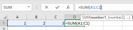
   You can also use this technique to extend numeric or date series: if you have consecutive cells with 1, 2, 3, highlight all three cells and drag the dot to extend the numeric sequence to whatever end value you wish.

   You cannot use it to extend letter series, but you can repeat letter patterns: if you extend A-B-C over six new cells, you won’t get A-B-C-D-E-F-G-H-I, but instead A-B-C-A-B-C-A-B-C.

   You can even select all three of the examples in Blank 1 and drag them at once. Excel interprets each series appropriately.

   Note: You can change some of your options with the Auto-fill Options icon that appears after you finish the fill: choose to copy instead of extending a series; choose to fill without formatting; choose to fill the formatting only; etc. Click the Auto-fill icon to browse its options.

   This works with both Windows machines and Macs, but only for cells continuous with the one you want to copy. Also, for the Blanks 2 exercise in the next sheet, you would have to repeat this for each category you need to fill in.

Proceed to the Blanks 2 sheet. Think about scale: imagine having to repeat this action if you had thousands of cells in different categories like this to fill.

1. • (PC) Home Tab, Editing > Find & Select > Go to Special > Blanks > OK * (Mac) Edit Menu > Find > Go To…> Special… > Blanks > OK * Type =, then hit the up directional arrow. Hit CTRL+Enter (PC) or ⌘+Enter (Mac)

Cell References

In each of our formulas so far, we’ve referred to cells like this:

=A1

to indicate the first row of column A. When we copy or drag this reference one cell to the right it becomes B1, or if we drag it one cell down, it automatically becomes A2.

Sometimes we don’t want our references to change as we drag our formulas, though. Absolute references provide unchanging references by placing a $ before the column letter and row number:

=$A$1

The reference above will stay the same no matter where we move it.

VLOOKUP

Module 4 Video: VLOOKUP (18:13 minutes)

(View the VLOOKUP sheet.)
The VLOOKUP function provides a way to merge or join additional data into a dataset, using a common code or value.

Here’s an example of a VLOOKUP function:

=VLOOKUP(A3,$F$3:$G$9,2,FALSE)

Let’s take a closer look at what each element of the function means:

Value	Parameter	Description
A3	lookup_value	Value in our main table that we’re looking to match in the other table
$F$3:$G$9	table_array	The other table we need information from (lock references with $)
2	col_index_num	The column from the other table we’re looking for
FALSE	[range_lookup]	Whether you want approximate matches [TRUE] or exact matches [FALSE]

VLOOKUP can refer to a value in a different sheet or even a different workbook on your computer. If you click into a cell on the other table while filling out your VLOOKUP formula, it will automatically supply the reference necessary to link to the other sheet or workbook.

(View the Ex_Main sheet for a second, more complex VLOOKUP exercise which will look up a second table located in the Ex_Lookup sheet.)

XLOOKUP

VLOOKUP (and its corollary function, HLOOKUP) will eventually be replaced by a new function called XLOOKUP. The most recent versions of Excel on Mac, PC, and online include XLOOKUP and VLOOKUP, but older versions (e.g. 2016, 2019) only use VLOOKUP. We’ll cover XLOOKUP in future semesters. If you’re interested in learning more, see the official documentation for XLOOKUP.

Introduction to PivotTables

Module 5 Video: PivotTables (23:01 minutes)

(View the second Excel spreadsheet, Pivot_Tables_IPEDS.)

Pivot_Tables_IPEDS.xlsx

PivotTables create cross-tabulations displaying values split out across categories displayed as row and/or column headings. Make sure you have only one cell or the entire table selected to ensure Excel auto-detects your data correctly.

Windows: Insert Tab>PivotTable

Mac: Go to Data Tab>PivotTable>Create Manual PivotTable…

Adding data: Click and drag to areas at the bottom of “PivotTable Fields”. Remove by dragging back to list.

Go ahead and drag the category State to the Rows area, and Control of Institution to the Columns box. Finally, click to select the very last variable in the list, Endowment (per FTE enrollment). It should appear in the Values box as “Sum of Endowment (p…,” but you can change the value that appears there. Click on it to see the menu, Value Field Settings. You could choose Average to make your pivot table look like the example below. We’ll talk about this more in a minute.

Columns and Rows: The categories on the edges of the PivotTable

• Multiple categories on a single axis will be nested

Values: The numbers shown in the cells of the PivotTable (each cell summarizes one variable for the group defined by the combination of its column and row categories.)

In most cases, there will be many rows in your dataset represented by one cell in your PivotTable, so we need to summarize or aggregate the data. In the example above, there are many public or private universities in each state.

Aggregation of Values

• Click on the field in the Values area and choose “Value Field Settings” in the window that appears to change the default aggregation.
• “Summarize Values By” determines the mathematical function used to summarize the cells
  • Frequencies are available via the Count function. Note: this will not count missing values.
  • Exercise: Compare Frequency of “Control of Institution” using Count on “Control of Institution” and a Count on “Applicants Total”.
    1. Drag “Control of Institutions” to Rows.
    2. Drag “Control of Institutions” to Values, and make sure it is summarized by “Count of”
    3. Drag “Applicants Total” to Values, and make sure it is summarized by “Count of”
• “Show Values As” allows more complex calculations based on other cells (e.g. percent of total)
• Mac: Click the “i” icon on the Value. “Show Values As” is located under the “Options»” tab.

Sorting and Filtering Columns and Rows

• Use the arrows at the right of “Row Labels” and “Column Labels”
• “More Sort Options” provides advanced sorting by Values (Mac: Not Available)
  • Advanced filtering available in “Label Filters” and “Value Filters”

Filters

• Dragging a field to the Filters area will create a drop-down filter at the top of the sheet.

PivotTable Exercises

1. What are the “Enrolled Totals” in public and private schools (see “Control of Institutions”)?
2. Which “Geographic Region” has the highest average “ACT Composite 75th Percentile Score”? How many regions have average scores below the national (Grand Total) average?
3. Which category of “Degree of Urbanization” contains the most public (“Control of Institution”) universities?
   1. What percent of the “Applications Total” go to each of the top two “Degrees of Urbanization”? (Hint: Use the Show Values As tab in Values Field Settings)

Next Steps:

Other Useful Tools to Explore in Excel:

• Pivot Charts: PivotTables with added visualizations.
• Power Query (Windows-only): Loading and filtering large datasets
  • Data Tab > Get & Transform
• Data Validation: Control data entry to prevent errors
  • Data Tab > Data Validation
• Macros: Record and re-use processes, or write your own code

Getting Help:

• LinkedIn Learning through UNC provides training videos (free to UNC students) on a wide variety of Excel functions. (See the login link on the right side of the UNC Software Distribution page.)
• Carolina Talent provides similar resources to Faculty and Staff.
• Data Carpentry - Spreadsheets
• Michele Hayslett of the Davis Library Research Hub is available for one-on-one consultations.
• Matt Jansen of the Davis Library Research Hub is available for one-on-one consultations.

Data Sources:

• World Development Indicators (Excel_Workshop.xlsx)
• IPEDS (Pivot_Tables_IPEDS.xlsx), accessed here.

SOLUTIONS

Disclaimer: For many of these questions, there are multiple ways to get to the correct values. These are merely one way you could get the desired results.

Completed Companion Excel Workbook

Companion Excel Workbook with all exercises completed with formulas and pasted values.

Pivot Tables Exercises

1. What are the “Enrolled Totals” in public and private schools (see “Control of Institution”)?
   • Drag “Control of Institutions” to Row Labels to layout the table
   • Drag “Enrolled Total” to Values
   • Click “Enrolled Total” in Values and select Value Field Settings…
   • Change Summarize Values to Sum instead of the default Count
2. Which “Geographic Region” has the highest average “ACT Composite 75th Percentile Score”? How many regions have average scores below the national (Grand Total) average?
   • Drag “Geographic Region” to Row Labels
   • Drag “ACT Composite 75th Percentile Score” to Values
   • Click “ACT Composite 75th Percentile Score” to Values and select Value Field Settings…
   • Change Summarize Values by to Average. * Sort the table by clicking the arrow icon in the corner of Row Labels on the table itself (see arrow)
   • Click More Sort Options, then select Descending (Z to A) and set to “Average of ACT Composite 75th Percentile Score”

1. Which category of “Degree of Urbanization” contains the most public (“Control of Institution”) universities?
   • Drag “Degree of Urbanization” to Row Labels. Drag “ID number” to Values.
   • Click “ID Number” in Values, then Value Field Settings > Summarize Values by to set aggregation to Count.
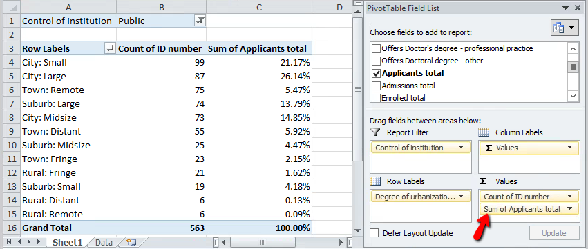
   • Note: ANY variable that doesn’t have missing values will work here. The Count aggregation is essentially counting the number of filled cells in the given categories. So some values will have slightly different counts due to empty cells. * Drag “Control of Institution” to Report Filter. Use the Filter appearing at the top of the screen to select “Public”. * Use the Row Labels arrow, then More Sort Options to sort by “Count of ID Number”
     1. What percent of the “Applications Total” go to each of the top two “Degrees of Urbanization”? (Hint: Use the Show Values As tab in Value Field Settings)
   • Assume that we keep the Public filter active. Leave the earlier work in place.
   • Drag “Applicants Total” to Values and place it under “Count of ID number”.
   • Click “Applicants Total” and select Value Field Settings
     • Under Summarize Values by, choose sum
     • Under Show Values As, choose % of Column Total

This site is open source. Improve this page.